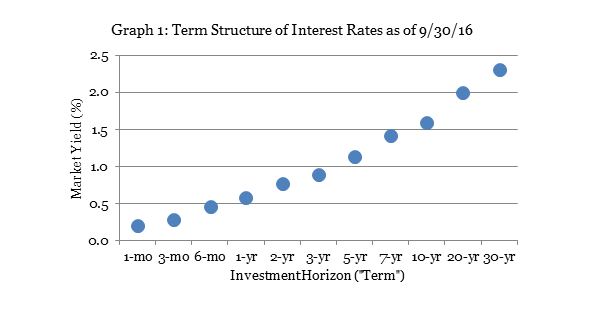
You probably know something about the term structure of interest rates: that is, the relationship between the market interest rate and the investment horizon (or “term”). An upward-sloping term structure of interest rates, for example, means that long-horizon bonds are offering higher rates or yields than short-horizon bonds—as, for example, Graph 1 shows was true for U.S. Treasury bonds on September 30.
Other investment metrics have term structures, too. One of the most important is the term structure of correlations between any two assets. Correlation measures the degree to which the returns for a pair of assets move together; it is estimated by taking the string of returns observed over some available historical period for a pair of assets and plugging them into the following equation:
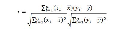
It’s important to notice that the formula doesn’t specify the investment horizon over which the returns should be measured: is it daily returns? Monthly? Quarterly? Annual? It could be even shorter (minutes or seconds, for example) or even longer (such as two-year periods, or even decades). Actually any of them is correct, but here’s the really crucial point: your choice of an investment horizon matters when you estimate a correlation coefficient, and exactly how it matters gives you a valuable piece of investment information. (Okay, maybe that’s two crucial points.)
To see this, use the total returns for any two assets over any historical period: for example, exchange-traded Equity REITs (FTSE NAREIT All Equity REIT Index) and the broad U.S. stock market (Russell 3000 Index) over the 36-year period from 9/30/1980 through 9/30/2016. Divide up the overall historical period into sub-periods any way you wish: for illustration I used 144 quarterly returns, 36 annual returns (remember that “annual” doesn’t have to be the same as “calendar-year”), 18 two-year returns, and 9 four-year returns. Now compute the correlation coefficients using each of the investment horizons:
- The estimated correlation in quarterly returns has been 63%
- The estimated correlation in annual returns has been 57%
- The estimated correlation in two-year returns has been 51%
- The estimated correlation in four-year returns has been -31%
Which estimate is correct? All of them. Well, then, which one should you use in your investment decision-making? The one that best matches your own investment horizon. For example, if you’re a day-trader, then what you really care about is how closely the returns on two assets move together on a day-by-day basis—so you should estimate their correlation using daily returns. (Similarly, if you’re a high-frequency trader, you care about co-movements over periods of seconds or even less.) On the other hand, if you make trading decisions on a monthly basis, what’s relevant to you is the correlation in monthly returns; if your investment decisions tend to take place quarterly, you care about the correlation in quarterly returns. And if (like me) you’re a buy-and-hold investor and measure your investment horizon in years or decades, then a correlation coefficient based on monthly or quarterly data is irrelevant: you need to know how closely two assets move together over periods measured in years or decades.
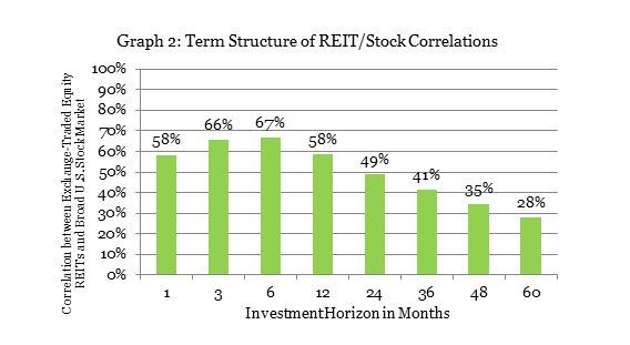
Now let’s back up a bit: in the above example I estimated the correlations using non-overlapping periods of each length—just for exposition—but that’s not a requirement; in fact, you can get a more accurate picture of the entire term structure of correlations by using overlapping periods of each length. Graph 2 shows the term structure of correlations between exchange-traded Equity REITs and the Russell 3000 using overlapping periods from the end of 1989 through September 2016. (The reason this analysis starts at the end of 1989 is because that’s when sector returns—discussed in the next paragraph—became available.) You can see that the REIT-stock correlation declines very steadily from 67% measured using semiannual (6-month) investment horizons to just 28% measured using five-year (60-month) investment horizons.
You’ve probably heard about the creation of the new “Real Estate” sector as part of the Global Industry Classification Standard (GICS®). Graph 3 shows one of the most important reasons for that change: the correlation between exchange-traded Equity REITs and the S&P Financial sector has actually been quite low—especially over the longer investment horizons relevant for most investors (just 36% over five-year horizons)—even though Equity REITs have been categorized within the Financial sector all this time!
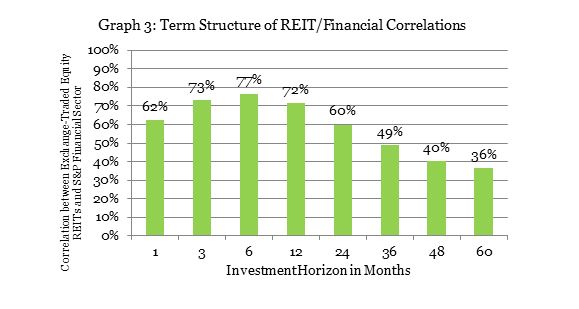
Those declining term structures of correlations mean that the diversification benefits of exchange-traded Equity REITs are even greater—relative to the broad stock market, or relative to the Financial sector in which they were trapped for so long—for investors with a long horizon than for those focused on short-term results.
Now, what does the slope of the term structure of correlations tell us about the relationship between two assets? There are two reasons that a correlation could be high: because the two assets share the same set of underlying return drivers, or alternatively because there are sources of “spillover” that cause their returns to move together more closely than their return drivers do. Conversely, there are two reasons that a correlation could be low: because the two assets respond to different sets of return drivers, or alternatively because problems—such as difficulties measuring returns accurately—cause their observed returns to be different from the underlying true returns based on their return drivers.
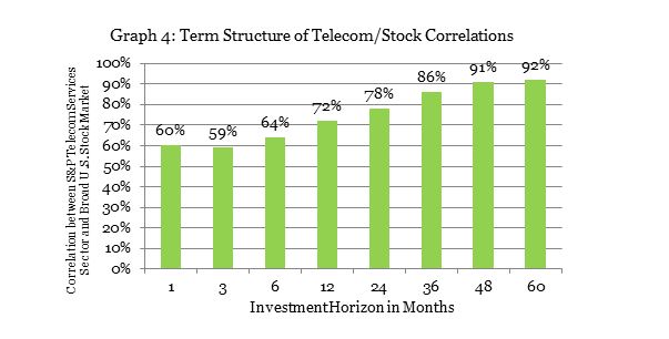
The slope of the term structure can help us distinguish between the two explanations. Consider Graph 4, which shows the same analysis as in Graph 2 but this time looking at the term structure of correlations between the S&P Telecom Services sector (rather than Equity REITs) and the broad U.S. stock market. While the term structure of REIT/Stock correlations was very strongly downward-sloping, the term structure of Telecom/Stock correlations is very strongly upward-sloping. The interpretation of this is that short-term movements in the Telecom sector may develop differently than short-term movements in other sectors of the stock market, but long-term returns for Telecom stocks are driven by the same underlying set of market conditions that drive the returns of companies in almost every other segment of the stock market: namely, the business cycle. The fact that the correlation over five-year periods is as high as 92% means that it doesn’t really matter whether an investor in (most of) the stock market gets his exposure to the business cycle through Telecom stock investments or through (most) other stock investments: the exposure is to the same set of long-term return drivers regardless.
In contrast, the interpretation of the downward-sloping term structure of correlations shown in Graph 2 (and Graph 3) is that “spillover” between the REIT and non-REIT segments of the stock market causes stock prices to move together over short periods; over longer investment horizons, though, the returns on Equity REITs are driven by an entirely different set of market conditions than those that drive returns in the rest of the stock market: namely, the real estate market cycle, which is entirely different from the business cycle. For example, investors who think of Equity REITs as financial companies may buy or sell Equity REITs based on short-term developments relevant to banks—that’s spillover—but, after some time, other investors will notice that such ill-informed trading has caused Equity REITs to become over- or under-valued relative to conditions in the real estate market and will trade in the opposite direction, causing the correlation over longer horizons to fall.
One last graph helps to drive home the importance of interpreting the slope of the term structure of correlations: Graph 5 shows the term structure of correlations between exchange-traded Equity REITs and returns measured on the unlisted side of the real estate market using the NCREIF Property Index. (The NPI measures unlevered returns for institutionally-owned core real estate in the U.S. on the basis of property appraisals. Several other indices of unlisted real estate—including those for private equity real estate funds following core, value-add, or opportunistic strategies, as well as those based on transaction prices rather than appraisals, produce essentially the same picture.)
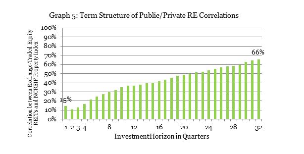
The term structure of public/private real estate correlations is strongly upward-sloping—in fact, even more strongly upward-sloping than the term structure of Telecom/Stock correlations shown in Graph 4, increasing from just 15% using quarterly returns to 66% using returns measured over eight-year (32-quarter) horizons. The reason is this: property values are extraordinarily difficult to estimate with any accuracy—and they are generally estimated only about once each year because of the expense—so the returns measured in the illiquid real estate market during any given quarter are notoriously divorced from actual returns during that quarter. (Those measurement problems on the illiquid side, incidentally, are part of the reason that REITs are frequently able to take advantage of public/private arbitrage to increase their own company values.) Long-term returns on illiquid real estate investments, however, are driven by exactly the same set of market conditions as long-term returns for exchange-traded Equity REITs: namely, the real estate market cycle.
To simplify the process of constructing and managing an investment portfolio, strategic decisions should be based on return characteristics over the long-term investment horizon relevant to that investor: that is, retirement investors, pension funds, endowments, foundations, and other long-term investors should use correlations estimated from returns measured over years or decades, not months or quarters, to develop their broad investment strategy. Tactical decisions will naturally be made using short-term market conditions—but tactical decisions, of course, are generally made on the basis of transitory mis-valuations rather than correlations anyway. Tactical decisions may focus, for example, on which company’s stock to buy today because that company’s stock is undervalued today, while strategic decisions have to do with how much of the overall portfolio should go into each of the fundamental asset classes (stocks, bonds, real estate, and cash), and those decisions—like the definition of the asset class itself—must be based on long-horizon tendencies rather than fleeting short-horizon performance.